Introduction to the problem and rationale:
Neurodegeneration leads to the continued deterioration in the function of neurons or death of the neurons. Among hundreds of neurodegenerative disorders, the top 4 prevalent disorders are, Amyotrophic Lateral Sclerosis (ALS), Alzheimer's disease (AD), Huntington's disease (HD) and Parkinson's disease (PD). Increasing growth rate of aging people is one of the most significant factors for rise in the number of people with a neurodegenerative disorder.
Looking at developed countries, as per US Parkinson foundation, there will be over 1 million PD patients in US alone by 2020, a number larger than total patients with multiple sclerosis, muscular dystrophy and ALS. While the National Institute of health reports growth rate of 50,000 new patients every year. Worldwide nearly 10 million people are estimated to be affected by PD. PD prevalence is likely to be twofold by 2030. In these estimates, one should also factor in the lesser amount of awareness and diagnosis in developing countries.
With these numbers, the diagnosis and treatment for PD have a lot to achieve and improve. PD care suffers from lack of early diagnosis which could control the progression and stop irreversible damage. PD patient care is also constrained by insufficient, sporadic symptom monitoring and lesser access to specialist care globally. The infrequent encounters with healthcare professionals lead to intuitive decision-making and risk misdiagnosis. For the patient it results in hampered quality of life (QoL) and high-end expenditures of therapy, medications and surgery at times.
Hence, timely prediction of patients at risk of PD can help with more befitting and personalized treatment planning.
How can AI help with Parkinson’s disease?
TotemX labs aims to show that Machine learning (ML) and Internet of Things (IoT) can help restrain the impact of this chronic disease with early diagnosis and continuous symptom monitoring. Use of widely available tools like computers, smartphones, digital assistants and wearable sensors facilitates high frequency data collection and management. Tests like walking, voice, tapping and memory can be devised as an ML application on smart devices to manage PD. In present chapter, current scenario in PD care is discussed and to improve it, practical ML implementations using voice and tapping data are demonstrated.
Current methods of Parkinson's disease diagnosis and treatment modes:
A useful list of early warning signs of PD is compiled by Mayo Clinic is as follows-

Parkinson’s clinical testing methods:
Unlike most diseases, PD cannot be detected by blood tests or regular lab tests. Standard method for diagnosing PD is performing a clinical assessment of motor symptoms. However, the probability of absence or varying severity of the symptoms of PD during the clinical assessment may lead to incorrect observations. For example, many cases motor impairment appears much later to cognitive symptoms causing much of neurological damage.
Second test is by administering Levodopa and check for a positive response which is again subjective to individual patient response and of course the unsolicited side effects.
Another level of confirmation is possible with brain scans, magnetic resonance imaging (MRI), Computed tomography (CT), Positron emission tomography (PET) and DaTscan.
Early symptoms largely coincide the effects of aging. In addition, PD symptoms also resemble to other neurodegenerative or non-neurodegenerative conditions, making the exact identification difficult.
Parkinson’s disease treatment:
It is needless to mention that the disease has no cure till date and unfortunately the treatment involves only controlling the symptoms and progression through medicines, therapies and surgery.
For more than 5 decades, the symptomatic treatment of PD aims to reduce the declining levels of the neurotransmitter dopamine with the orally administered dopamine precursor, levodopa (Brand name Sinemet). MAO-B inhibitors is another category to tackle Dopamine breakdown. Though the severe adverse effects on motor performance resulting from such medicine defeat the very purpose.
PD patients are prone to develop fluctuations in motor and/or cognitive functions as side effects, e.g. levodopa induced Dyskinesia, levodopa induced Psychosis, vomiting and so on. Deep brain simulations or surgery are the options depending on the stage of the patient when medications are not effective enough.
Identification of the stage and severity of the disease is carried out by the Movement Disorder Society-Unified Parkinson’s Disease Rating Scale (MDS-UPDRS) and Hoehn and Yahr (HY) Scale.
Concerns and challenges:
Challenges in early diagnosis of Parkinson’s disease:
The accuracy of PD tests in clinical setting has been varying based on the individual expertise level and human bias. Approx. 25% of PD diagnoses are incorrect when compared to post-mortem autopsy. Sadly, in certain cases the putamenal Dopamine is depleted to nearly 80%, and around 60% of SNpc dopaminergic neurons have already been lost, before physical symptoms are detectable (in terms of conventional diagnosis criterion). Please feel free to reach us to read our original research chapter that covers more depth and has and list of sources, if interested.
While the Levodopa challenge predict 70-81% cases, researchers suggest it to be redundant and trust the physical-neurological tests more. Not to mention the uncertain risk of subjecting the patient to unnecessary side effects.
Among the scan tests, MRI tests are next level recommendation for cases where the primary symptoms cannot be ascertained. PET requires to subject the patient to a radioactive substance injection to check the abnormalities of Dopamine transmission. CT scans create a 3D picture for the doctors with main aim to rule out other conditions and not direct diagnosis of PD. DaTscan, another radioactive IV scanning test can only confirm a prognosis and not make first-hand diagnosis of PD. In addition, it has limitations in distinguishing PD with other Dopamine depleting disorders. Given the cost to effectiveness trade-off combined with the administration complexity, these tests are more suitable for later stages and not for early diagnosis.
Thus, requirement of simple yet effective diagnostic tools to capture early signs as depicted in previous figure, is evident.
Concerns and challenges in treatment of Parkinson’s disease
In the treatment area, the options are limited. The primary option is medication as explained above. The dosage is decided based on clinical assessment, HY scores and MDS-UPDRS scoring system. Correct identification of severity and stage (patient profiling) is crucial to ensure the patient is not under-medicated or over-medicated.
Application of machine learning in solving Parkinson’s disease diagnosis and treatment challenges:
It has been a popular belief that ML requires a large database, state-of-art computing facilities and knowledge of complex algorithms.
Contrary to that, TotemX Labs proposes solution with small sized and medium sized public datasets, to build a proof of concept.
We create easy-to-implement models. There is a vast variety of applications of ML in PD. In the proposal a few examples are discussed in order to open the discussion for larger arena of possibilities.
Basic machine learning cycle workflow:
For the purpose ease-of-understanding for the medical or non-technical readers, we depict the very basic steps of the process.

This figure represents the generic process flow of a typical Machine Learning model, excluding advance steps of MLOPs, as not applicable in the present usecase. It starts with raw data acquisition from user. To make data understandable, we need to extract features from the data which can be fed further to ML algorithm. So, in the next step the data is cleaned and preprocessed. In feature engineering, we remove unnecessary features as well as create some new features which would help with training the ML model. The dataset with selected features is split in Train and Test dataset, where Test dataset is reserved for evaluation and prediction purpose. The Train dataset is further split for validation purpose. ML model is trained on Train dataset and validated with validation dataset. Once model is finalized the predictions are made for Test dataset, which are provided to user. From feedback of users and predictions the model is improvised with more data and/or better ML algorithms.
Data acquisition
Biomarkers are essential for accurate and early diagnosis of any disease or disorder. Advancement of health-tech has made obtaining biomarkers less complicated nowadays. The collected biomarkers data have become tools to drive ML applications in healthcare. In this chapter our particular focus is non-invasive biomarkers data to develop ML model for diagnosis of PD. In case of PD some of the non-invasive biomarker resources are human voice, finger movements, imaging etc.
Biomarkers dataset selection factors for Parkinson’s disease prognosis
The selection of these datasets has been made based on factors such as -
- Ease and cost of data acquisition,
- Type and size of data,
- Continuous data update,
- Amount of clinical attention required and
- Requirement of physical visit to clinic by patient
The evaluations are tabulated as below-

Voice and Keystrokes datasets are simpler and cheaper to obtain. The features and amount of data can be continuous which can facilitate regular improvements to the ML model. Since human voice and typing keystrokes can be recorded from anywhere, no physical visit to clinic is required. Data interpretation and analysis can be accomplished with minimal expert assistance.
Data preprocessing
The data recorded from any medium, e.g. sensors, needs to be converted in machine comprehensible form. Data cleaning is the first step carried out to remove unnecessary data and outliers. It is very important to identify significant data required for particular problem. For example, there is a possibility of corrupt or missing data fields which should be eliminated. Consequently, transformation of data i.e. attributes selection, scaling and normalization of the data is done. Sometimes in the case of large dataset the size of the data is reduced to save on computational efforts.

Feature engineering
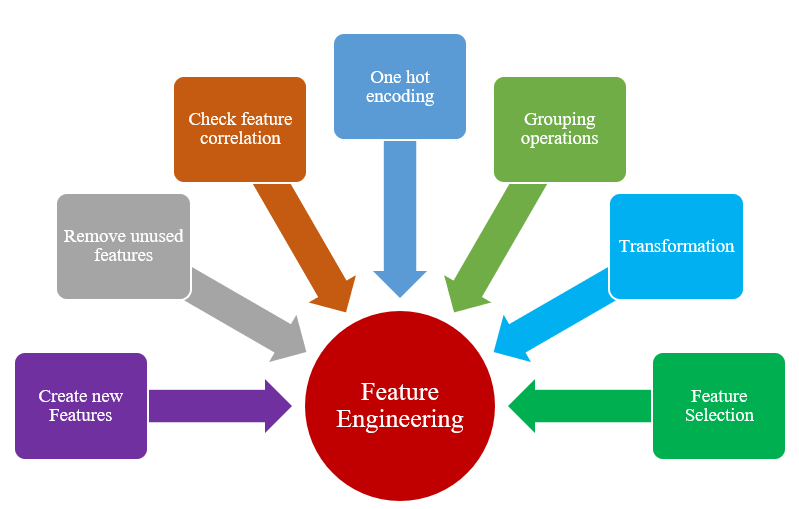
Feature engineering is one of the most important processes in ML workflow. Feature engineering can make or break an ML model. This is the part where domain knowledge can be helpful.
Feature engineering makes data interpretable for ML algorithms. Creating new features, removing unused features, checking correlation of features, one-hot encoding categorical features, detecting outliers, grouping operations, transformation of features are part of feature engineering process. Feature selection impacts the model performance significantly. The selection is made using different feature combinations, feature importance and model evaluation.
Train Machine Learning models
Before training ML model, feature engineered data is split into Train and Test datasets to reserve a data subset for final evaluation of the model. Training dataset is further divided with validation set for Cross Validation (CV) purpose. Since it is not completely straightforward to choose an apt ML model, general practice should be training dataset through multiple machine learning algorithms. There are many impressive ML open source libraries consisting various algorithms available. Some popular libraries and algorithms are Support Vector Machine (SVM), Linear and Logistic Regression, K-Nearest Neighbors (KNN), Naïve Bayes, Tree Regressors, Boosted Tree Regressors and Neural Networks.
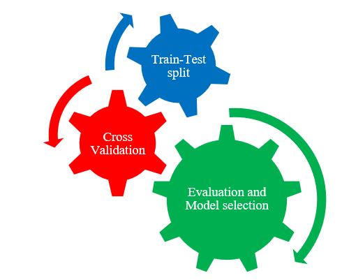
Next in the process a few selected algorithms are cross validated and compared using technique such as K-fold CV method. More details on K-fold CV and ML algorithms are covered in Example 1: Voice data based early diagnosis. In cases of insufficient accuracy or overfitting/underfitting, any/all the processes of more data acquisition, data preprocessing and feature engineering are repeated, and models are retrained.
Machine learning evaluation and predictions
On the basis of the evaluation from cross validation and test dataset, we can employ an ideal ML candidate (algorithm) to predict on future input data. The evaluation metrics are picked according to problem definition and output requirements. Some of the popular metrics are Root Mean Squared Error (RMSE), Mean Absolute Error (MAE), Log Loss, Accuracy, F1-Score, Confusion Matrix, Area Under Curve (AUC), Matthews Correlation Coefficient (MCC) etc. The test datasets in present chapter are evaluated with accuracy, sensitivity, specificity and MCC.
For mathematical explanations please reach us to receive access to entire research chapter.
Continuous improvement
There is no perfect or 100 % accurate ML model. Continuous improvements can be rendered by recurrent cycle fetching more data, creating better features, employing advanced ML algorithms and training more robust ML models.
Implementation: Machine learning for Parkinson’s disease early prediction
Given the data security compliances, on-going treatment data is usually not made public. Open secured data sharing would help improving the treatment globally. However, such policy issues are already under discussion in Healthcare arena, hence are not made part of this chapter.
With two detailed diverse diagnosis examples on open datasets, the authors provide a practical beginner’s guide of ML in PD care for healthcare professionals. Although, a conceptual summary of existing implementations in treatment would also be provided to motivate the readers in that direction.
EXAMPLE 1: VOICE DATA BASED EARLY DIAGNOSIS OF PARKINSON'S DISEASE
Approximately 90% percent of PD patients exhibit some form of vocal disorders in the earlier stages of the disease. Due to the decrease in motor control that is the hallmark of the disease, voice can be used as a means to detect and diagnose PD. The main reason behind the popularity of PD diagnosis from speech impairments is gathering speech samples and doing signal processing of their voice has low cost and it is appropriate for telemonitoring and telediagnosis systems. The interest in diagnosis of PD through vocal tests has grown over the years. One can refer to know almost all the relevant research done so far.
Objective
To show that how simple it is to develop a predictive binary classification ML model to distinguish PD patients from healthy controls using only human voice.
Solution
To build voice-based ML classification model and explain the general ML workflow, outcome and future possible improvements. Two datasets, different ML classifier algorithms and corresponding evaluation metrics are discussed.
Data acquisition - voice data
In this example we have acquired open source voice datasets available on UC Irvine Machine Learning Repository.
Dataset I has structure as follows-
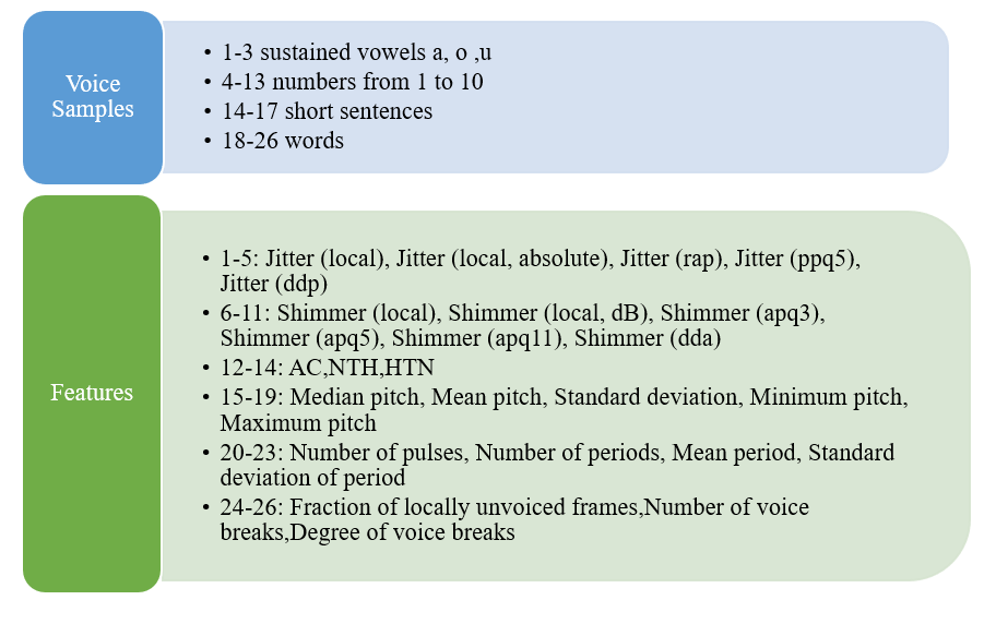
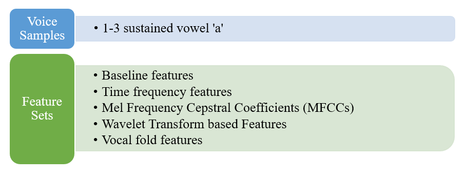
Dataset II has following format-
Data preprocessing
Both the datasets are carefully collected and structured by the researchers. Hence no data cleaning is required. Moreover, datasets are considerably small, so data reduction is necessary either. As a part of data preprocessing, first step is to identify the data into feature columns as X and labels (also called target variable) as y. Feature columns X are already defined in data acquisition section. Here in both the datasets, y consists labels ‘0’ for healthy controls and ‘1’ for patients with PD. X contains all type of features where we may have numeric values in different units or scale. For example, in dataset (I) some Jitter features have values ranging from 10-1 to 10-5 whereas some pitch features are of 102. Hence scaling and normalization of X is performed. Also, for some of the ML algorithms to produce predictions correctly, normalization and scaling of the data is advised. We have labeled ‘Class’ data column as y in both the datasets. All the X feature columns are scaled/normalized using a function from open source library called scikit-learn.
Feature Engineering
Both the datasets are created with the help of domain experts and therefore there are very well curated features in the dataset. As a result, we will not have to deal with many of the processes in feature engineering. Some of the features such as patient ID which do not contribute to prediction of PD/healthy label and so have been dropped. Since there are no categorical variables/features, one-hot-encoding is considered.
For dataset (II), there are 750+ features, out of which we will select only certain number of features. We will start by taking only Baseline features for initial model development. We will include a greater number of features and observe the change in output. Our aim is to demonstrate the simplest way of building a PD classification model with ML, complex feature selection technique details are avoided. We will also present results with all the features. Although it is usually recommended to perform feature selection and include only most important features in the final model. Significant amount of Feature Engineering shall be covered in Example 2: Tappy keystroke.
Train Machine Learning models
Train-Test split and Cross Validation
It is a methodological mistake to train the model to learn the parameters of a prediction function and testing it on the same data. Such model leads to a situation called overfitting. In this situation model would not predict correctly on yet unseen data. To avoid it, firstly we will split our feature engineered data into two datasets. Namely Train dataset and Test Dataset. Test dataset is the unseen dataset on which we verify our model performance before deploying the model into system. In our case we have split the dataset into 80% Train and 20% Test.
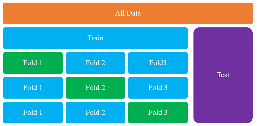
Cross-validation (CV) is a technique applied in machine learning to find better performing ML estimate how the model is expected to perform in general when used to make predictions on data not used during the training of the model. For this we held out some more part of the training dataset in terms of validation dataset. However, this may cause available training samples reduced to the amount which is not sufficient for learning the model. K-fold Cross Validation provides a solution to this issue by splitting the training data into k number of folds. This method is very useful for dataset with small number of samples.
The procedure for k-fold CV is as follows-
Machine Learning Classification Algorithms
As there is no all-powerful medicine for all the disease, there is no one-for-all ML classifier algorithm for every classification problem. We have implemented and compared some of the most effective and industry standard ML classifiers. We will give brief introduction of the algorithms we have used here. Theoretical and practical literature of all these algorithms is openly available.
I. Support Vector Machine (SVM): SVM, formally defined by a separating hyperplane, is a supervised ML algorithm which can be used for both classification or regression problems. It is believed that it works very good for classification of small dataset. For given labeled training data, SVM outputs an optimal hyperplane which categorizes new examples. In case of binary classification this hyperplane is a line dividing a plane in two parts where in each class lay in either side.
II. Logistic Regression (LR): LR is the go-to method for binary classification problems. Logistic regression transforms its output using sigmoid function to return a probability value. Logistic regression models the probability of the default class (e.g. the first class). For example, to predict person has PD or not, then the first class could be PD patient and the logistic regression model could be written as the probability of PD patient given a person’s age. The older person will have higher probability of having PD than younger person.
III. K-Nearest Neighbors (KNN): KNN is a classifier algorithm where the learning is based on assumption that similar things are near to each other. The standard steps of KNN are -
- i. Load the data
- ii. Calculate distance (Euclidian) from the new data to already classified data
- iii. Based on distance values do the sorting
- iv. Pick k top sorted values (value of k is defined by user)
- v. Count the frequency of each class that appears and select the class which appeared the most
- vi. Return the value of selected class
IV. Multi-layer Perceptron (MLP) Classifier: MLP uses a Neural Network to perform classification. NN consists of at least three layers, namely input layer, hidden layer and output layer. MLPs are mainly involved in two motions, forward and backward. In the forward pass, the input is fed from the input layer through the hidden layers to the output layer, and the prediction is measured against the true labels. In the backward pass, using backpropagation is used to move the MLP one step closer to the error minimum. This is executed with algorithm such as stochastic gradient descent. This is repeated until the state known as convergence (lowest error possible) is achieved.
V. Random Forest (RF): RF is probably the most popular classification algorithm. The underlying concept for RF is based on decision tree classifier. In other words, decision trees are building blocks of RF. Unlike above mentioned algorithms, RF is ensemble learning method. Unlike above mentioned algorithms, RF is ensemble learning method. RF is an ensemble of individual decision trees. Usually a greater number of trees leads to higher accuracy. Simple example: let’s say we have features [x1, x2, x3, x4] with corresponding targets/labels as [y1, y2, y3, y4]. From the input features RF would generate three decision trees [x1, x2, x3], [x1, x2, x4], [x2, x3, x4] and prediction is based on the majority of votes from each of the decision trees created.
VI. Extreme Gradient Boosting (XGBoost): Similar to RF, XGBoost is also an ensemble learning method. It has recently been dominating applied machine learning due to it speed, performance and scalability. XGBoost is the gradient boosting decision tree implementation. XGBoost algorithm is parallelizable so it can harness the power of multi-core computers. It is parallelizable onto Graphics Processing Unit (GPUs) too which enables it to train on very large datasets as well. XGBoost provides inbuilt algorithmic advancements like regularization for avoiding overfitting, efficient handling of missing data and cross validation capability. Reader may refer the XGBoost library documentation for more details and practical implementation.
Except XGBoost, all the above algorithms are implemented from scikit-learn library. In machine learning, a hyperparameter is a parameter whose value is initialized before starting the training of model. Since hyperparameters govern the training process, all of the mentioned algorithms accomplish better results with hyperparameters tuning. We are going to implement all the classifiers with default hyperparameter values only.
Evaluation and Prediction
The ultimate goal of ML classifier is to classify new and unseen data with maximum number of correct predictions. As explained earlier, to get robust prediction model we execute K-fold CV first on training data. The metrics we use for CV are accuracy, precision, recall, F1-score and Matthews Correlation Coefficient (MCC). With k=10 value in K-fold CV, we calculate all the metrics for 10 folds. From all these folds, for each metric, mean value is obtained. We run K-fold CV for all the above referred ML classifiers. The mean value of each metric is computed for every classifier. An apt ML classifier can be selected based on the mean values of the metrics and can be applied on the Test dataset to verify the model learning.
In this example we have applied all the described ML algorithms on the Test dataset to show the comparison of their performance with different data size, quality and number of features, number of samples etc.
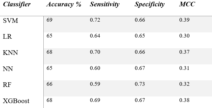
Results for Parkinson's Speech Dataset I with Multiple Types of Sound Recordings
Results for Parkinson's Speech Dataset II with Multiple Types of Sound Recordings
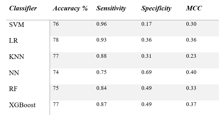
With increased number of features, in Table below we see some better performance of classifiers on the test data. SVM, LR and KNN are still suffering with low specificity and MCC. NN, RF and XGBoost have performed quite better with increased number of features (56 features). Finally, taking all the feature sets (750+) and evaluating NN, RF and XGBoost.

A few points to consider developing binary classifier for PD patient diagnosis-
- More and effective data samples can help to improve performance of classifier such as sustained vowels such as ‘a’.
- Metrics sensitivity, specificity and MCC are good indicators for selecting a right classifier
- More features certainly help the performance of some ML classifiers like NN, Random Forest and XGBoost. Although trade-off like computation cost and overfitting should be considered.
- For scalable prediction system algorithms such as NN and XGBoost are good choices
- Employing IoT devices such as mobile or digital assistants (Google assistant, Amazon Alexa) can help collecting data as well as diagnosing PD using ML/AI powered app
NOTE: The current version does not include the Tappy stroke dataset predictions and methodological discussion, which was also conducted under the research.The present version is kept concise for web. For more interpretation or discussions on the results, please contact us.